Frequentist and Bayesian Hypothesis Testing: An Intuitive Guide for Urologists and Clinicians

Abstract

Given the limitations of frequentist method for null hypothesis significance testing, different authors recommend alternatives such as Bayesian inference. A poor understanding of both statistical frameworks is common among clinicians. The present is a gentle narrative review of the frequentist and Bayesian methods intended for physicians not familiar with mathematics. The frequentist p-value is the probability of finding a value equal to or higher than that observed in a study, assuming that the null hypothesis (H0) is true. The H0 is rejected or not based on a p threshold of 0.05, and this dichotomous approach does not express the probability that the alternative hypothesis (H1) is true. The Bayesian method calculates the probability of H1 and H0 considering prior odds and the Bayes factor (Bf). Prior odds are the researcher's belief about the probability of H1, and the Bf quantifies how consistent the data is concerning H1 and H0. The Bayesian prediction is not dichotomous but is expressed in continuous scales of the Bf and of the posterior odds. The JASP software enables the performance of both frequentist and Bayesian analyses in a friendly and intuitive way, and its application is displayed at the end of the paper. In conclusion, the frequentist method expresses how consistent the data is with H0 in terms of p-values, with no consideration of the probability of H1. The Bayesian model is a more comprehensive prediction because it quantifies in continuous scales the evidence for H1 versus H0 in terms of the Bf and the posterior odds.

Resumen

Dadas las limitaciones del método de significancia frecuentista basado en la hipótesis nula, diferentes autores recomiendan alternativas como la inferencia bayesiana. Es común entre los médicos una comprensión deficiente de ambos marcos estadísticos. Esta es una revisión narrativa amigable de los métodos frecuentista y bayesiano dirigida quienes no están familiarizados con las matemáticas. El valor de p frecuentista es la probabilidad de encontrar un valor igual o superior al observado en un estudio, asumiendo que la hipótesis nula (H0) es cierta. La H0 se rechaza o no con base en un umbral p de 0.05, y este enfoque dicotómico no expresa la probabilidad de que la hipótesis alternativa (H1) sea verdadera. El método bayesiano calcula la probabilidad de H1 y H0 considerando las probabilidades a priori y el factor de Bayes (fB). Las probabilidades a priori son la creencia del investigador sobre la probabilidad de H1, y el fB cuantifica cuán consistentes son los datos con respecto a H1 y H0. La predicción bayesiana no es dicotómica, sino que se expresa en escalas continuas del fB y de las probabilidades a posteriori. El programa JASP permite realizar análisis frecuentista y bayesiano de una forma simple e intuitiva, y su aplicación se muestra al final del documento. En conclusión, el método frecuentista expresa cuán consistentes son los datos con H0 en términos de valores p, sin considerar la probabilidad de H1. El modelo bayesiano es una predicción más completa porque cuantifica en escalas continuas la evidencia de H1 versus H0 en términos del fB y de las probabilidades a posteriori.

Keywords

null hypothesis testing - bayesian analysis - Bayes factor - frequentist - statistical analysis - p-value - dichotomization - bayesian hypothesis testing - null hypothesis significance testing - JASP

Palabras Clave

prueba de hipótesis nula - análisis bayesiano - factor de Bayes - frecuentista - análisis estadístico - valor p - dicotomización - prueba de hipótesis bayesiana - prueba de significación de hipótesis nula - JASP

Introduction

Many scientific publications base their quantitative analyses on null hypothesis significance testing and p-values, a theoretical framework developed almost a century ago by Ronald Fisher,[1] Jerzy Neyman, and Egon Pearson.[2] However, an increasing number of authors have pointed out the limitations of this so-called ‘frequentist’ approach, mainly related to the low reproducibility of the studies.[3] [4] [5] [6]

In 2018, three major urological magazines, the Journal of Urology, the British Journal of Urology, and European Urology, published the ‘Guidelines for reporting of statistics for clinical research in urology’, which state that we should not continue describing the studies as ‘positive’ or ‘negative’ according to p-values.[7] [8] [9] They encourage all researchers to follow the American Statistical Association statement on p-values, published in 2016,[10] which declares that the probability that a hypothesis is true does not depend on the p-value, and scientific conclusions should not be based on specific p-value thresholds. The referred document proposes alternatives like Bayesian estimations and methods that emphasize estimation over testing, among others.[10]

Despite the mentioned publications, problems related to the frequentist and Bayesian hypothesis test methods remain difficult to understand for many physicians who are not familiar with statistics and mathematics.[11] In light of this, the present narrative review offers an intuitive explanation of the subject. Throughout the text, the concepts are exemplified by comparing the mean International Prostate Symptom Score (IPSS) between two groups.

Frequentist Hypothesis Testing

Sampling Distribution and Sampling Error

Sampling distribution and sampling error are essential concepts to understand the frequentist method. The sampling distribution is the hypothetical distribution of data from samples obtained from a population.[12] [13] [14] [15] [16] Suppose a hypothesis testing to compare the mean IPSS between a group of patients who take medicine A and a group who take medicine B. The population is the entire group of people about whom we want to carry out the study, and is defined by the inclusion and exclusion criteria. Say we draw different samples over and over from the population to compare the effect of medicine A and medicine B. We will obtain a value (a difference between means, dm) from each one of these samples. The sampling distribution is the curve obtained from these values ([Figure 1]).

Fig. 1 Sampling distribution. The circle on the left shows the population (P) or group of people suitable to take medicine A or B, according to inclusion and exclusion criteria. In the center, each small circle corresponds to a sample obtained from the population. Each letter corresponds to individuals who take medicine A or medicine B. We obtain a difference between means (dm) from each sample, which is the difference between the mean IPSS with medicine A and the mean International Prostate Symptom Score (IPSS) with medicine B. On the right, the results are grouped in a curve, which is the sampling distribution curve. In the example, the curve is normal, but in other scenarios it might have a different configuration.

The frequentist method is based on the assumption that there are no differences between the groups in the population. Therefore, in the case of a dm, the frequentist considers that the population parameter is zero (the null hypothesis, H0, is true). If that is the case, and we draw different hypothetical samples from a population (in which H0 is true), we would expect in each one of them a difference between groups equal to zero. However, most results will be different from zero due to the so-called sampling error: the inaccuracy of working with a sample and not with the entire population.[17] [18] [19] We can build a hypothetical sample distribution curve despite the sampling error thanks to statistical methods and mathematical laws. The ‘law’ for a dm says that the sampling distribution curve will be Gaussian, the mean will be zero, and most samples will fall around zero. These features are part of the Central Limit Theorem, described more than 200 years ago, and applied when sample sizes are larger than 60[16] [20] ([Figure 2] depicts an example).

Fig. 2 The Central Limit Theorem. The circle on the left shows the population (P) of patients suitable to take medicine A or medicine B. Hypothesis testing assumes that in this population there are no differences between the mean IPSS with medication A and the mean IPSS with medication B (that is, the dm is equal to zero: H0 is true). In the center, we draw many samples with at least 60 individuals (n ≥ 60) from the population P. We calculate in each sample a dm between A and B, which is not necessarily zero, due to the sampling error. On the right, all the differences (dm) obtained are grouped in a sampling distribution curve, which will have a normal distribution. The mean of the curve is equal to the difference in means in the population P, that is, zero.

Obtaining and Understanding the p-value

Unlike the examples in [figure 1] and [2], researchers do not work with the entire population or with many different samples, but with a single sample. Once the result is obtained, it is placed into the hypothetical sampling distribution curve thanks to statistical methods such as the Student t-test. That is possible because we can predict the shape of the sampling distribution curve, as discussed before. Then, we calculate the percentage of hypothetical samples with an equal or higher value under the sampling distribution curve: this percentage is the p-value. The p-value is the probability of finding the same result or higher within the hypothetical sampling distribution curve, assuming that the sample comes from a population with no differences between the two groups, that is, assuming that H0 is true[11] [12] [13] ([Figure 3]). The p-value is a conditional probability because its calculation depends on the assumption (condition) that H0 is correct and does not indicate the probability that H0 is true, as many erroneously think.

Fig. 3 Calculation of the p-value, one tale test. The circle on the left shows the population P of patients suitable to take medicine A or B. We assume no differences between the two groups in the population (that is, the dm is zero: H0 is true). In the center, a sample is obtained, with a size ≥ 60. We obtain a dm from the sample. On the right, according to the Central Limit Theorem, it is known in advance that the hypothetical sample distribution follows a normal curve and has a mean equal to the population mean, which is zero. Thanks to these premises, the Student t statistical test enables the location of the study's result within the sampling distribution curve. Also, we calculate the percentage of hypothetical samples whose results are equal to or higher than the result obtained in the studied sample. The percentage mentioned is the p-value. In the example, the percentage was of 15%, that is, p = 0.15.

Suppose we conduct a single study to compare medication A and medication B in terms of the mean IPSS, and the difference obtained is 5 points. Then, we apply the Student t-test to place the outcome in the sampling distribution curve. Say the result is at one end of the sampling distribution curve, and from that point are located 15% of the possible hypothetical samples: the p-value, in this case, is 0.15. In other words, if we assume that there are no differences between the two groups in the population, and we perform the study repeatedly, 15% of the studies will show a difference of 5 points or more ([Figure 3]).

A p-value of 0.05 means that the sample is at an extreme of the sampling distribution because only 5% of the theoretical studies carried out in the population will show a similar result or higher. Traditionally, 0.05 is the threshold to suspect that the H0 is less likely to be the case, and there are actual differences between the two groups in the population, namely, the population parameter is not the null value (the alternative hypothesis, H1, is true).[13] The 0.05 threshold is called the level of statistical significance.[11] [12] [13] [21]

The p-value is usually reported along with a 95% confidence interval (CI). As aforementioned, the sample estimate might be different from the population parameter due to the sampling error. The 95% CI expresses the inaccuracy caused by the sampling error and is a range in which the population parameter might lie.[22] If we draw samples over and over from the population, 95% of them will have a CI that contains the population parameter.[22] [23] For example, if the population parameter is a dm = 3 (H1 true), and we obtain an infinite number of samples from the population, for 95% of these samples the 95% CI will contain the value 3. It is wrong to state that there is a probability of 0.95 that the 95% CI contains the population parameter. The probability of 0.95 refers to the proportion of infinite samples whose CI contains the population parameter and does not apply to a single CI.[22]

The p-value dictates how rare it is to obtain a value equal to or higher than the outcome of a single study if we assume no real differences between the groups compared in the population. Unfortunately, the p-value does not answer the fundamental question: what is the probability of a difference in the population between the compared groups? The frequentist method focuses on the wrong question: given a population with no differences between the groups, what is the probability of a result equal or more extreme than the one obtained? The real question is: given the data, what is the probability of a real difference between groups in the population? (What is the probability of H1?) As we discuss now, the Bayesian method offers the answer.

Bayesian Hypothesis Testing

Bayesian statistics calculate the probability that an event is true considering the results obtained (the data) and the knowledge that one has of this probability before developing a study (the prior probability). It is based on the Bayes theorem, formulated by Thomas Bayes, an 18th-century English statistician.

The Bayesian framework deals with conditional probability, which is the probability of an event given that another event has occurred.[24] [25] Conditional probability is expressed as p(A | B), and means ‘the probability of A, given that B occurs’. Bayes' theorem enables us to find a conditional probability when we are provided with its inverse: if we know p(A | B), we can calculate p(B | A).[25] That is the case of hypothesis testing: we seek the probability of a hypothesis given the data p(H | data), and our data (the result of our study) enables us to retrieve the probability of the data, given the hypothesis p(data | H). In the example mentioned before of medicine A versus medicine B, we want to know if there is in the population a difference in terms of the IPSS given the outcome of a study [p(H1 | data)], and the study provides the probability of the outcome obtained if we assume that H1 is true [p(data | H1)].

Bayes formula for two rival hypothesis (H1 and H0) is expressed in the form of odds:[26]

p ( H1 ∣ data ) p ( H1) p ( data ∣ H1 )

-------------------------------- = -------------------------- X ------------------------

p ( H0 ∣ data ) p ( H0 ) p ( data ∣ H0 )

posterior odds for H1vsH0 prior odds for H1vsH0 Bayes Factor

In words, the posterior odds of H1 versus H0 given the data is the product of the prior odds for H1 versus H0 times the Bayes Factor (Bf). We can turn odds into probability (p) by applying the formula p = odds/1 + odds.[27] The prior odds are what we believe before the study about the probability of H1 versus H0. The Bf is equal to the probability of the data, given H1, divided by the probability of the data, given H0, and represents the strength of evidence that the data provide for H1 versus H0. For example, if we think a priori that the rival hypotheses have the same probability [p(H1)/p(h0) = 0.5/0.5 = 1], and the Bf is 20 (that is, the observed data is 20 times more likely under H1 than under H0), the posterior odds are 1 × 20 = 20. Then, we turn odds into probability: p = 20/20 + 1 = 0.95, and we conclude that the data has increased the probability of H1 from 0.5 to 0.95. Note that, unlike the frequentist method, this time we have answered the main question: what is the probability of H1?

Prior Odds

Prior odds are researcher beliefs about how plausible are the hypotheses.[27] [28] [29] [30] It is background knowledge that is relevant when we make any conditional prediction, not only in hypothesis testing. For instance, suppose two 65-year-old male patients with a prostate-specific antigen (PSA) level of 5 ng/ml. They live in the same geographical area. We want to know the risk of prostate cancer given the PSA. The first man is white, does not have a family history of prostate cancer, and his prostate volume is of 80 mL. The second man is black, has a family history of prostate cancer, and his prostate volume is of 20 mL. Despite their similar PSA level (the data), the black man has a higher probability of developing prostate cancer because of his higher pretest odds.

Prior odds are a subjective way to quantify uncertainty and depend on the result of previous studies in the field, theoretical considerations, biological plausibility, and basic physiological knowledge.[28] [29] [31] [32] When there is skepticism towards H1, the researcher assigns low prior odds that H1 is true. When it is more plausible, the prior odds will be high. A study that compares a new selective alpha-blocker and placebo to treat lower urinary tract symptoms secondary to prostatic enlargement, for example, will have high prior odds in favor of H1 because the benefit of alpha-blockers in this scenario has been previously proven.

Bayes Factor

The Bf is a comparison of how well two hypotheses predict the data. It is a measure of how likely the data is in a hypothesis compared to another hypothesis.[28] [32] Therefore, the Bf is not a probability but a ratio of probabilities.[33] For instance, if the Bf = 10 when we compare H1 versus H0, data are 10 times more likely to have occurred under H1 than under H0.

The English statistician Sir Harold Jeffreys proposed a classification of the evidence for a hypothesis in terms of specific Bf intervals[28] ([Table 1]). According to the scheme, the Bf describes ‘anecdotal’, ‘moderate’, ‘strong’, ‘very strong’, or ‘extreme’ relative evidence for a hypothesis. This set of rigid labels facilitates scientific communication, but there is no specific threshold to prefer H1 and reject H0.[28] [30] [34] The Bf does not yield a dichotomous decision (reject or not reject H0) but a relative comparison of the hypothesis. Its value must be interpreted along with the prior probability to predict how likely is H1. Most Bayesian studies describe the Bf but not the prior odds nor the posterior odds to enable the reader to make their own conclusions according to their beliefs.

Table 1 Evidence categories for the Bayes Factor in favor of the alternative hypothesis (H1) over the null hypothesis (H0)[28]

Bayes Factor	Interpretation
> 100	Extreme evidence for H1
30–100	Very strong evidence for H1
10–30	Strong evidence for H1
3–10	Moderate evidence for H1
1–3	Anecdotal evidence for H1
1	No evidence
0.33–1	Anecdotal evidence for H0
0.33–0.1	Moderate evidence for H0
0.1–0.03	Strong evidence for H0
0.03–0.01	Very strong evidence for H0
< 0.01	Extreme evidence for H0

The Bf depends on three elements: data likelihood, the prior distribution, and the H0 specification.

Data likelihood. Likelihood is a term used to describe the probability of observing data that have already been collected.[25] [27] Suppose a study comparing the mean IPPS between an alpha-blocker and placebo with a final result of 10 points. The parameter, in this case, is the dm. Data likelihood estimates the probability of our data given the infinite possible values of the parameter. If we consider dm = 10 points, the probability of the study's outcome (our data, 10 points) will be high. If we consider dm = 5 points, the probability of the outcome (our data, 10 points) will be low. We make the same calculation for every possible value of the parameter to draw a likelihood profile curve (also called likelihood function curve).[23] [27] [35] The curve says how likely is the data for every value of the parameter. [Figure 4] illustrates the example.

Fig. 4 Likelihood profile curve for a dm. The x-axis is the unknown parameter dm. We calculate how likely are different values of dm given an observed dm = 10. The parameter value dm = 10 has the highest likelihood. The parameter value dm = 5 has a low likelihood.

The prior distribution. A primary characteristic of the Bayesian method is the uncertainty about the value of the population parameter, unlike the frequentist analysis, in which the parameters are considered fixed.[36] When we calculate the sample size for a frequentist comparison between means, we assume that the dm is exactly 0 for H0 and has an exact prespecified value for H1. The Bayesian comparison between means, instead, assumes uncertainty about those values. In the case of the H1 parameter, we assign a range of possible values. The distribution of those values is called the prior distribution.[23] [28] [37] Common sorts of prior distribution are normal distribution and t-distribution ([Figure 5]).

Fig. 5 Examples of prior distributions. The x-axis corresponds to the parameter values. The y-axis, the density, refers to how frequent is each parameter value.

A common mistake is considering the Bayesian parameters ‘random’, in opposition to the fixed point by the frequentist.[36] The parameter in the Bayesian model is not random but uncertain. Uncertainty in the Bayesian method is usually misinterpreted as ‘randomness’.[36]

There are two different ways to choose the prior distribution in Bayesian analysis.[27] [28] [38] [39] The first is the subjective way, which is based on the researcher's beliefs about the parameters. These beliefs are supported by previous theoretical information, and the prior distribution is therefore called ‘informative’. The informative distribution describes a specific range for the parameter with the more possible values. The second is the objective way, not based on the researcher's beliefs, which yield a ‘non-informative’ distribution. It is called objective because there is no bias toward any specific value: the distribution displays a wide range of values of the parameter because all of them are equally likely, or almost equally likely, from the researcher's point of view. For instance, if we plan to compare the difference in the mean IPPS between a new alpha-blocker and placebo, and a previous meta-analysis describes a difference of 10 points, we can set an ‘informative’ prior distribution centered on 10 and with a narrow standard deviation. If there is no previous information about the topic, we would have to set a ‘non-informative’ prior with a wide range of values for the difference in means ([Figure 5]).

Different authors advocate non-informative priors, especially for scenarios in which there is no previous reliable information about the research topic.[28] [40] [41] In that sense, ‘default’ priors are recommended. ‘Default’ prior non-informative distributions are prior distributions with limited preference for particular parameter values. They are recommended because they increase the objectivity of the analyses and facilitate communication, because they provide a standard reference to compare Bfs from different studies.[42] [43] The flat prior (uniform prior, with no biases towards any parameter value) is a sort of non-informative distribution not recommended because it leads to Bfs in favor of the H0 even if the data suggest a difference in favor of the H1.[23] [40] [44] Therefore, non-informative priors adopted by researchers span a wide range of parameter values but are not entirely flat. The Cauchy distribution is the default prior for the t-test, and it is similar to the Gaussian normal distribution but has fatter tails and less central mass[28] [29] [38] [40] [42] ([Figure 5]).

It is important to emphasize two concepts. First, the prior distribution must be specified before (not after) the data collection.[23] [28] [29] [39] [40] Once the researcher knows their study's data, the prior distribution's construction is prone to bias.[29] [39] However, redefining the prior distribution is allowed during data obtention if additional information becomes available.³⁹ Second, the prior odds and the prior distribution are not the same.[28] [41] The prior odds are the researcher's prior beliefs about the probability of H1 in relation to H0. The prior distribution is a range of possible values of the parameter in H1, assigned by the researcher.

H0 specification. In Bayesian analysis, the H0 is usually described as a single fixed point equal to zero (no differences between the groups).[28] [29] [37] [45] Conceptually, however, the Bayesian method acknowledges that considering H0, the population parameter is never exactly zero, but a value near zero; therefore, the specification of the H0 can be an interval around 0.[29] [37] [46]

The Posterior Distribution

The posterior distribution is the distribution of possible values of the H1 parameter obtained after updating the prior distribution based on the data.[23] [27] [28] [37] [38] [41] [42] It combines our beliefs before knowing the data (the prior distribution) and the information provided by the data (the likelihood).[28] In many cases, the information provided by the data can reduce the uncertainty of the H1 parameter.

The posterior distribution is calculated by multiplying the data likelihood by the prior distribution[23] [28] [37] [42] ([Figure 6]). The range obtained is described by central tendency measures such as mean, median, and mode.[28] The dispersion around the central tendency measurement is described with an interval that includes 95% of the parameter values.[28] The mentioned interval is called the 95% credible interval and means that we are 95% certain that the actual parameter value falls in the interval assuming that the alternative hypothesis is true (H1).[41] [42] Recall that the probability of a true H1 is not expressed by the credible interval nor the posterior distribution. As aforementioned, the probability H1 versus H0 is given by the posterior odds.

Fig. 6 Calculation of the posterior distribution. The posterior distribution (blue line) is obtained by the multiplication of the prior (dotted line) and the data likelihood (yellow line). CI = credible interval.

Calculation of the Bayes Factor

As aforementioned, the Bf is the probability of the data, given H1, divided by the probability of the data, given H0:

Bf = p(data | H1)/p(data | H0).

The probability of the data given H0 refers to how likely are the data given the parameter value of no differences (the point null), that is to say, the height of the likelihood profile curve for the point null.[28] [44] [45]

The probability of the data given H1 is a more complex calculation because H1 prior distribution is not a point null, but a range of values.[27] [28] [29] [44] In that sense, we need to integrate the data likelihood to H1 prior distribution, which is, in simple terms, multiplying (averaging) the prior distribution by the data likelihood for each parameter value and adding all the obtained values.[28] [47] The outcome is called H1 marginal likelihood.

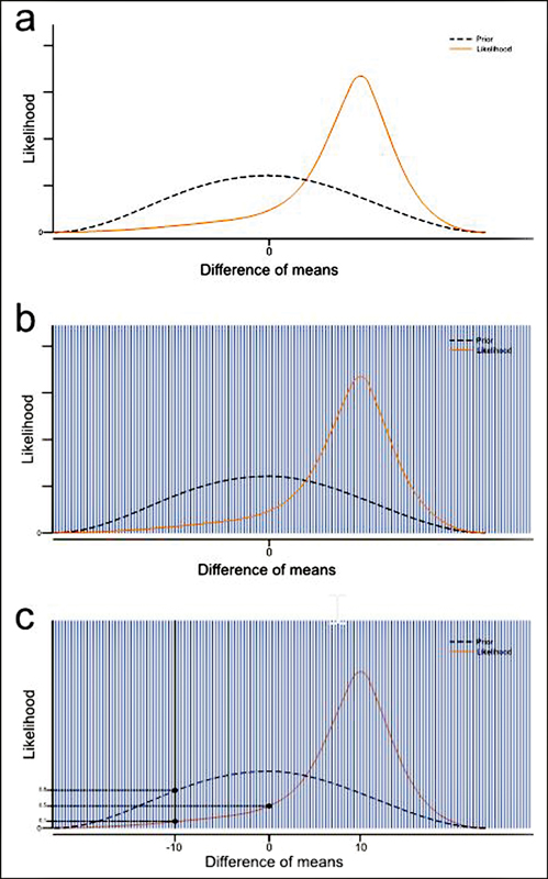
The Bf calculation based on the H1 marginal likelihood and point-null likelihood can be graphically illustrated (August 9, 2015 posting by Alexander Etz to ‘Understanding Bayes: Visualization of the Bayes Factor’ blog; unreferenced, retrieved from https://alexanderetz.com/2015/08/09/understanding-bayes-visualization-of-bf). The parameter's continuous distribution is interpreted as a set of many points spaced very close together. We calculate the likelihood ratio for every point and multiply the likelihood ratio by the respective H1 prior density. Then, we do the sum of all calculations, and finally, we divide by the total number of points ([Figure 7]).

Fig. 7 Calculation of the Bayes Factor (Bf). a) The x-axis is the parameter value (dm). The yellow curve is the likelihood profile curve, and the dashed curve is the prior distribution. b) The parameter's continuous distribution can be thought of as a set of many point hypotheses spaced very close together. c) We determine the likelihood ratio (LR) for the different dm point values relative to the point null (H0), and then we weight the LR on the prior distribution. The LR is the ratio of the heights of the likelihood curve (yellow curve). For instance, we calculate the LR for dm = −10 relative to H0. The height is 0.1 for dm = −10 and 0.5 for the point null, so LR = 0.1/0.5 = 0.2. The LR is multiplied by the density assigned to dm = −10 in the prior distribution to weight the LR based on the prior distribution. In the example, the density in the prior distribution for dm = −10 is 0.8, so the weighted LR = 0.2 * 0.8 = 0.16. A similar calculation must be done for every single dm point hypotheses values of the x-axis. The Bf is obtained by adding all the weighted LR and dividing by the total number of points.

An alternative way to obtain the Bf is by dividing the posterior distribution height by the prior distribution height at the null point, with no calculation of the H1 marginal likelihood[28] [45] ([Figure 8]). The method corresponds to the Savage–Dickey density ratio, and is suitable for nested models.[28] [45] [46] [47] [48] In hypothesis testing, we say that we have nested models when we can obtain H0 by constraining the parameters of H1;[48] in other words, when H0 is a subset of H1. That is the case for most Bayesian hypothesis testing because the ‘point null’ of H0 can be obtained from H1 by setting the parameter equal to 0.[28]

Fig. 8 Calculation of the Bf, the Savage–Dickey method. The Bf is the ratio of the heights of the orange dots, which correspond to the height at the null point of the prior and posterior distributions.

Bayesian hypothesis testing is also feasible for complex models with many parameters or non-precise prior distributions.[28] If that is the case, we can apply computational methods like the Markov chain Monte Carlo (MCMC) to obtain the posterior distributions over the parameters.[37] [48] [49]

Sensitivity Analysis

The main challenge of Bayesian analysis is its dependence on the prior distribution. As aforementioned, the Bf calculation takes into consideration the H1 prior distribution, and the latter is in some sense arbitrary. One way to prevent a misleading Bf is to collect appropriate knowledge to set the best informative prior, but that is not always possible.[28] A second alternative is the so-called sensitive analysis, in which we check how the Bf is affected by changes in the width of the prior distribution.[28] [30] [36] If the Bf does not fall below certain limits despite different prior widths, we can conclude that we have a reliable and trustworthy assessment. If we obtain a Bf of 40 in our study, meaning strong evidence in favor H1, for example, and then different width values do not yield a Bf below 10, we are confident about the robustness of our research outcome.

Stop Rule and Sample Size in Bayesian Hypothesis Testing

The frequentist analysis specifies the sample size, and the study cannot be finished until the planned number of participants has been included. Bayesian methodology, instead, does not specify a sample size, and the Bf can be monitored as the data come in.[29] [41] [50] Bayesian researchers are allowed to stop the study whenever they want, especially if the evidence is compelling.[50] For example, some authors plan to stop the research as soon as Bf ≥ 10. Other ways to establish limits are deadlines for the recruitment process or fixing a maximum number of participants per group (a ‘maximum sample size’, N).[29] [41]

Example with JASP

JASP is a free statistical software program developed by researchers from the University of Amsterdam. Its name is an acronym for Jeffreys Awesome Statistics Package, referring to Sir Harold Jeffreys, who played a central role in developing the Bayesian methodology. JASP can be easily downloaded at https://jasp-stats.org/download/, and it includes both frequentist and Bayesian tests. Different tutorials are available online, and a guideline has been published recently.[34] [40] [41]

Let us suppose a hypothetical new pharmacological treatment for lower urinary tract symptoms, different from the traditional alpha-blockers. Let us call this new product the ‘x-blocker’. There is biological plausibility from a physiopathological perspective, but we do not have previous research regarding the product. Suppose we conduct a clinical trial comparing the ‘x-blocker’ and placebo in benign prostatic hyperplasia (BPH) patients in terms of the IPSS after four weeks of treatment. These are the data, following a normal distribution, including 60 patients per group:

‘X-blocker’ group, IPSS, 60 patients: 12,8,13,7,13,12,14,8,11,10,5, 10,11,10,9,10,5,10,16,10,10,4,3,10,11,17,11,8,11,9,9,12,12,14,12,12,8,8,13,13,9,13,7,7,9,8,7,9,7,14,14,6,6,11,6,6,15,15,11,9. The mean is 10.0, and the standard deviation is 3.0.

Placebo group, IPSS, 60 patients : 13,10,6,12,11,12,14,9,11,12,13,4,17,3,12,8,12,9,3,12,16,11,12,10,12,12,11,14,5,4,19,11,13,15,15,11,8,7,14,2,11,13,13,10,10,13,16,16,17,18,13,11,12,9,12,13,15,16,7,13. The mean is 11.3, and the standard deviation is 3.7.

We can set the hypothesis in terms of the Cohen d (δ), which is a way to express the effect size when we compare means.[40] [41] Cohen d values indicate the difference between the two groups in standard deviations. Values around 0.2 and 0.5 are considered small and medium effects respectively. Vales ≥ 0.8 are considered a large effect. For example, Cohen d = 1.2 is a large effect and says that the groups compared differ by 1.2 standard deviations. Cohen d = 0 means no difference between the two groups. Therefore, H0 assumes δ = 0, and H1 assumes δ ≠ 0.

To obtain the frequentist comparison, we first load the data into JASP. Then, we select ‘T-test’ and click on ‘Classical independent samples T-test’. In the options panel, we click on ‘Student’ on the test option. Finally, we select our alternative hypothesis option: if we do not have a directional prediction about H0 versus H1, we choose ‘Group 1≠Group 2’. [Table 2] presents the results.

Table 2 Frequentist outcome of a hypothetical comparison of the IPSS between two groups. Independent samples t-test (Student t-test)

	t	p	Cohen d	95% onfidence interval for the Cohen d
				Lower	Upper
International Prostate Symptom Score (IPSS)	2.21	0.029	0.404	0.042	0.765

Note: The analysis was performed with the JASP software.

The p-value = 0.02 describes how rare is the result in a population with no differences between the groups: only 2% of hypothetical samples will have a similar or more extreme outcome. Since the data are unlikely given H0 and the p-value is lower than 0.05, we reject the H0. Cohen d = 0.4 equates to a small/medium effect. The 95% CI says that we are confident that the population's Cohen d value will fall within the interval 0.04-0.75 because that will be the case in 95% of samples if we redo the study many times. As aforementioned, the probability of H1 (the probability of a difference between the groups in the population) is not specified by the frequentist approach.

To perform the JASP Bayesian analysis, we go to ‘T-test’ and then to ‘Bayesian independent samples T-test’. In the options panel, we choose the alternative hypothesis option, ‘Group 1≠Group 2’. In the ‘Bayes Factor’ option, we choose ‘BF10’ to obtain a Bf in favor of H1 over H0 (the program offers the option ‘BF01’ if we prefer a Bf describing the evidence in favor of H0 over H1). In the ‘Prior’ option, we select the prior H1 distribution: since our example establishes a lack of solid background evidence about the ‘x-blocker’, we choose the default ‘Cauchy’ distribution. The default Cauchy is centered on zero with an interquartile range r = 0.70, meaning we are 50% confident that the actual effect size lies between Cohen d = -0.7 and Cohen d = 0.7. In the ‘Plots’ option, we click on ‘Prior and posterior’ and ‘Bayes factor robustness check’, and we obtain [figures 9] and [10].

Fig. 9 Bayesian outcome of a hypothetical comparison of the mean IPSS between two groups. The analysis was performed with the JASP software.

Fig. 10 Sensitivity analysis or Bf robustness plot of a hypothetical comparison of the mean IPSS between two groups. The analysis was performed with the JASP software.

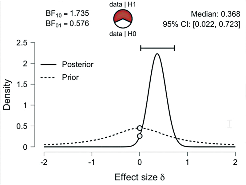
[Figure 9] features the main results of the Bayesian analysis. The BF10 is 1.73, meaning H1 predicts the data 1.73 times better than H0. The circle in red and white is called ‘the probability wheel’, and is a graphical representation of the Bf. The more evidence in favor of H1 (the higher the Bf, for example), the greater the red/white radius. The dashed line curve represents the Cauchy prior distribution, and the solid line curve represents the posterior distribution. Both curves present densities for different Cohen d values. The grey dots represent the height of the curves at the point null of no effect, and their values are used to calculate de Bf with the Savage–Dickey method, as aforementioned. The 95% CI = 0.02-0.7 refers to the 95% credibility interval, meaning a 95% probability that the population's Cohen d value falls in the interval, with a median of 0.36, as long as the H1 is true.

From the data of our example, we might predict the probability of H1. Suppose the researcher thinks the prior odds of the H1 versus H0 are 60/40. Given the obtained Bf = 1.73, the posterior odds of H1versus H0 are 60/40 × 1.73 = 2.59. We turn the posterior odds into probability (p) applying the formula p = odds/1 + odds = 2.59/1 + 2.59 = 0.72. The probability of a true H1 in our example is of 72%.

[Figure 10] displays a sensitivity analysis or Bayes factor robustness check. As seen, Bf lies in the interval 1-3 despite different Cauchy prior widths, meaning the Bf provides anecdotal evidence for the null hypothesis relative to the alternative hypothesis irrespective of the prior widths. The Bf decreases as the width is wider, indicating data with low robustness.

We can establish a parallel between the frequentist and the Bayesian method based on the example. The frequentist yields a dichotomous outcome accepting or rejecting H0: we rejected the null because the p-value was lower than 0.05. The probability of a real H1 cannot be determined. The Bayesian, instead, accepts uncertainty about H1 versus H0, and its prediction is continuous scales: the BF10 was 1.73, indicating anecdotal evidence in favor of H1, and the posterior probability of H1 was of 72%. The frequentist 95% CI says that 95% of repeated samples will have a CI that contains the population parameter, but we do not know if the obtained 95% CI (Cohen d: 0.04-0.76) corresponds to one of those samples. The obtained Bayesian 95% credibility interval, in turn, predicts that, in the case of a true H1, the population parameter lies between Cohen d 0.02-0.7.

Conclusion

The present manuscript synthesizes the main concepts of the frequentist and the Bayesian methodology. The frequentist approach has been used for many decades and is still the preferred method to analyze and report results despite its limitations related to the simplistic acceptance or rejection of the null hypothesis depending on the 0.05 p threshold, with no consideration of the probability of H1. Bayesian inference provides a compelling continuous measure of how likely is H1 in terms of the Bf and the posterior odds, and researchers should be encouraged to become familiar with this technique. Hopefully, the implementation of friendly tools like JASP will enable us to report Bayesian results more frequently, alone or in combination whit the frequentist conclusions.

Conflict of Interests

The authors have no conflict of interests to declare.

Acknowledgements

The authors would like to thank Christian Marin for his assistance during the design of the figures.

Financial Support

The authors declare they have received no financial support pertaining to the present article.

• References

• 1 Fisher RA. Statistical methods for research workers. Edinburgh (UK): Oliver and Boyd; 1934
• 2 Pearson K. On the Criterion that a Given System of Deviations from the Probable in the Case of a Correlated System of Variables is Such that it Can be Reasonably Supposed to have Arisen from Random Sampling. Philos Mag 1900; 50 (05) 157-175
• 3 Hopkins BL, Cole BL, Mason TL. A critique of the usefulness of inferential statistics in applied behavior analysis. Behav Anal 1998; 21 (01) 125-137
• 4 Goodman SN. p values, hypothesis tests, and likelihood: implications for epidemiology of a neglected historical debate. Am J Epidemiol 1993; 137 (05) 485-496 , discussion 497–501
• 5 Bakan D. The test of significance in psychological research. Psychol Bull 1966; 66 (06) 423-437
• 6 Ioannidis JPA. Why most published research findings are false. PLoS Med 2005; 2 (08) e124
• 7 Assel M, Sjoberg D, Elders A. et al. Guidelines for Reporting of Statistics for Clinical Research in Urology. Eur Urol 2019; 75 (03) 358-367
• 8 Assel M, Sjoberg D, Elders A. et al. Guidelines for reporting of statistics for clinical research in urology. J Urol 2019; 201 (03) 595-604
• 9 Assel M, Sjoberg D, Elders A. et al. Guidelines for reporting of statistics for clinical research in urology. BJU Int 2019; 123 (03) 401-410
• 10 Wasserstein RL, Lazar NA. The ASA Statement on p-Values: Context, Process, and Purpose. Am Stat 2016; 70 (02) 129-133
• 11 Westover MB, Westover KD, Bianchi MT. Significance testing as perverse probabilistic reasoning. BMC Med 2011; 9 (20) 20
• 12 Biau DJ, Jolles BM, Porcher R. P value and the theory of hypothesis testing: an explanation for new researchers. Clin Orthop Relat Res 2010; 468 (03) 885-892
• 13 Mark DB, Lee KL, Harrell Jr FE. Understanding the role of P values and hypothesis tests in clinical research. JAMA Cardiol 2016; 1 (09) 1048-1054
• 14 Lumley T, Diehr P, Emerson S, Chen L. The importance of the normality assumption in large public health data sets. Annu Rev Public Health 2002; 23 (01) 151-169
• 15 Altman DG, Bland JM. Statistics notes: the normal distribution. BMJ 1995; 310 (6975): 298
• 16 Pandis N. The sampling distribution. Am J Orthod Dentofacial Orthop 2015; 147 (04) 517-519
• 17 Altman DG, Bland JM. Uncertainty beyond sampling error. BMJ 2014; 349: g7065
• 18 Sedgwick P. A comparison of sampling error and standard error. BMJ 2015; 351: h3577
• 19 Ranstam J. Sampling uncertainty in medical research. Osteoarthritis Cartilage 2009; 17 (11) 1416-1419
• 20 Kwak SG, Kim JH. Central limit theorem: the cornerstone of modern statistics. Korean J Anesthesiol 2017; 70 (02) 144-156
• 21 Guyatt G, Jaeschke R, Heddle N, Cook D, Shannon H, Walter S. Basic statistics for clinicians: 1. Hypothesis testing. CMAJ 1995; 152 (01) 27-32
• 22 Sedgwick P. Understanding confidence intervals. BMJ 2014; 349: g6051
• 23 Bendtsen M. A gentle introduction to the comparison between null hypothesis testing and Bayesian analysis: Reanalysis of two randomized controlled trials. J Med Internet Res 2018; 20 (10) e10873
• 24 Etz A, Vandekerckhove J. Introduction to Bayesian Inference for Psychology. Psychon Bull Rev 2018; 25 (01) 5-34
• 25 Donovan T, Mickey R. Bayesian Statistics for Beginners. Oxford (UK): Oxford University Press; 2019
• 26 Kruschke JK, Liddell TM. The Bayesian New Statistics: Hypothesis testing, estimation, meta-analysis, and power analysis from a Bayesian perspective. Psychon Bull Rev 2018; 25 (01) 178-206
• 27 Cleophas T, Zwinderman A. Modern Bayesian Statistics in Clinical Research. Cham (Switzerland): Springer International Publishing; 2018
• 28 Lee M, Wagenmakers EJ. Bayesian Cognitive Modeling: a Practical Course. New York (NY): Cambridge Universtity Press; 2013
• 29 Andraszewicz S, Scheibehenne B, Rieskamp J, Grasman R, Verhagen J, Wagenmakers EJ. An Introduction to Bayesian Hypothesis Testing for Management Research. J Manage 2015; 41 (02) 521-543
• 30 Hoijtink H, Mulder J, van Lissa C, Gu X. A tutorial on testing hypotheses using the Bayes factor. Psychol Methods 2019; 24 (05) 539-556
• 31 van de Schoot R, Kaplan D, Denissen J, Asendorpf JB, Neyer FJ, van Aken MAG. A gentle introduction to bayesian analysis: applications to developmental research. Child Dev 2014; 85 (03) 842-860
• 32 Morey RD, Romeijn JW, Rouder JN. The philosophy of Bayes factors and the quantification of statistical evidence. J Math Psychol 2016; 72: 6-18
• 33 Goodman SN. Toward evidence-based medical statistics. 2: The Bayes factor. Ann Intern Med 1999; 130 (12) 1005-1013
• 34 Quintana DS, Williams DR. Bayesian alternatives for common null-hypothesis significance tests in psychiatry: a non-technical guide using JASP. BMC Psychiatry 2018; 18 (01) 178
• 35 Etz A. Introduction to the Concept of Likelihood and Its Applications. Adv Methods Pract Psychol Sci 2018; 1 (01) 60-69
• 36 Greenland S. Bayesian perspectives for epidemiological research: I. Foundations and basic methods. Int J Epidemiol 2006; 35 (03) 765-775
• 37 Kruschke JK. Bayesian estimation supersedes the t test. J Exp Psychol Gen 2013; 142 (02) 573-603
• 38 Rouder JN, Speckman PL, Sun D, Morey RD, Iverson G. Bayesian t tests for accepting and rejecting the null hypothesis. Psychon Bull Rev 2009; 16 (02) 225-237
• 39 Ferreira D, Barthoulot M, Pottecher J, Torp KD, Diemunsch P, Meyer N. Theory and practical use of Bayesian methods in interpreting clinical trial data: a narrative review. Br J Anaesth 2020; 125 (02) 201-207
• 40 Kelter R. Bayesian alternatives to null hypothesis significance testing in biomedical research: a non-technical introduction to Bayesian inference with JASP. BMC Med Res Methodol 2020; 20 (01) 142
• 41 van Doorn J, van den Bergh D, Böhm U. et al. The JASP guidelines for conducting and reporting a Bayesian analysis. Psychon Bull Rev 2021; 28 (03) 813-826
• 42 Keysers C, Gazzola V, Wagenmakers EJ. Using Bayes factor hypothesis testing in neuroscience to establish evidence of absence. Nat Neurosci 2020; 23 (07) 788-799
• 43 Wagenmakers EJ, Marsman M, Jamil T. et al. Bayesian inference for psychology. Part I: Theoretical advantages and practical ramifications. Psychon Bull Rev 2018; 25 (01) 35-57
• 44 Masson MEJ. A tutorial on a practical Bayesian alternative to null-hypothesis significance testing. Behav Res Methods 2011; 43 (03) 679-690
• 45 Wagenmakers EJ, Lodewyckx T, Kuriyal H, Grasman R. Bayesian hypothesis testing for psychologists: a tutorial on the Savage-Dickey method. Cognit Psychol 2010; 60 (03) 158-189
• 46 Morey RD, Rouder JN. Bayes factor approaches for testing interval null hypotheses. Psychol Methods 2011; 16 (04) 406-419
• 47 Heck DW. A caveat on the Savage-Dickey density ratio: The case of computing Bayes factors for regression parameters. Br J Math Stat Psychol 2019; 72 (02) 316-333
• 48 Kruschke JK, Liddell TM. Bayesian data analysis for newcomers. Psychon Bull Rev 2018; 25 (01) 155-177
• 49 Hamra G, MacLehose R, Richardson D. Markov chain Monte Carlo: an introduction for epidemiologists. Int J Epidemiol 2013; 42 (02) 627-634
• 50 Rouder JN. Optional stopping: no problem for Bayesians. Psychon Bull Rev 2014; 21 (02) 301-308

Publikationsverlauf

Eingereicht: 22. Juni 2022

Angenommen: 22. Juni 2022

Artikel online veröffentlicht:
28. September 2022